New Haven: Artifacts of Plans from a Cultural Past
The Semblance, Convergence and Resilience of the Nine Squares
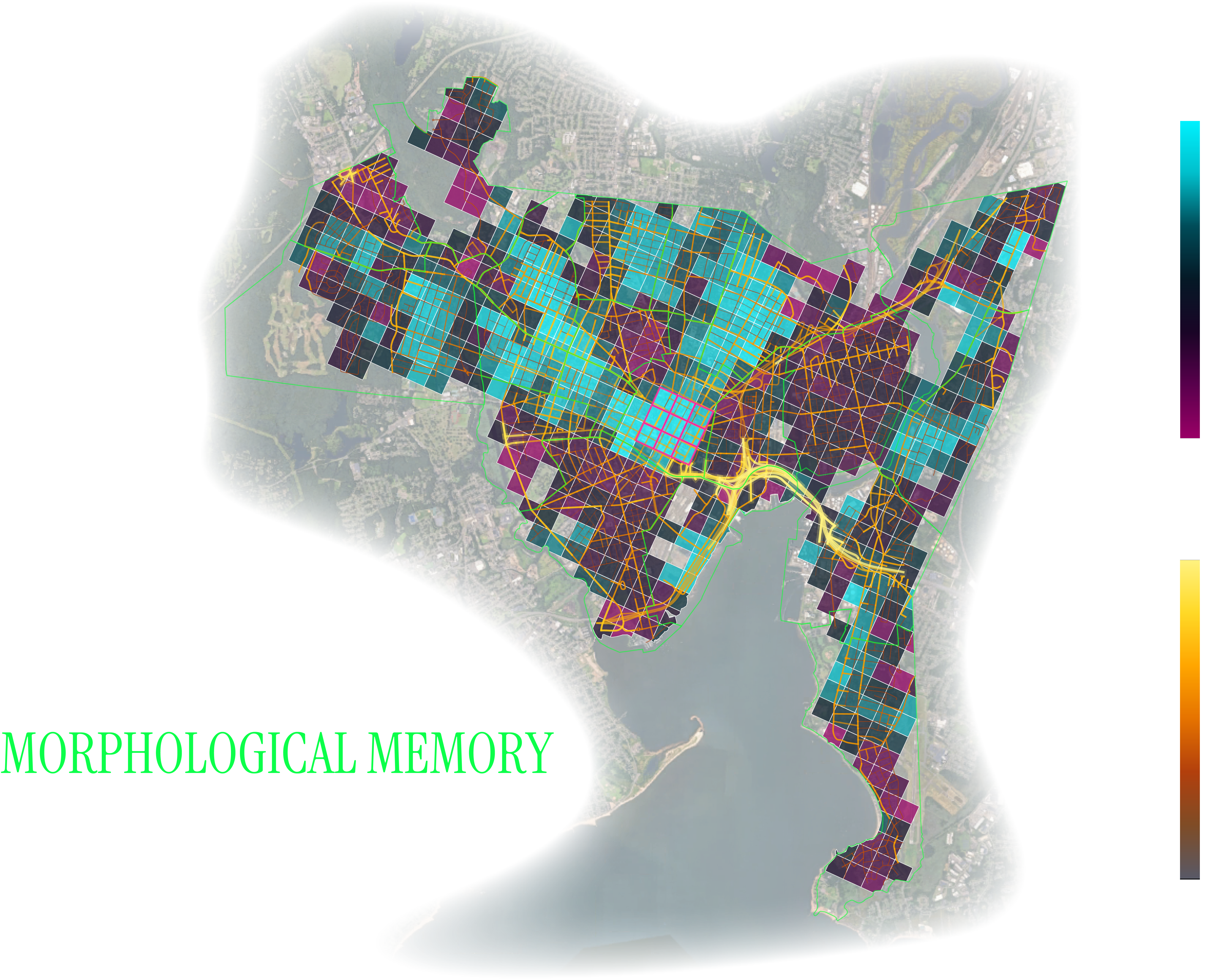
New Haven, founded in 1638, was planned around a 3×3 grid of squares — one of the earliest planned urban layouts in North America. As the city developed outward from this core, the original grid morphed into different typologies: curvilinear suburban streets, irregular industrial networks, and highway-era superblocks. The question is whether — and where — the memory of the original grid persists in the modern street network.
This project measures how much each part of the modern city "remembers" that original grid by imposing an expanded grid derived from the nine squares and computing street pattern similarity per cell.
acquisition
Acquire the full street network for New Haven from OpenStreetMap via osmnx. The network comprises 2,054 nodes and 5,305 edges with highway classification tags, projected to EPSG:32618 (UTM Zone 18N).
identification
Locate the spatial pattern of the nine-square grid by snapping to the 16 street intersections that define the 3×3 array (Grove, Elm, Chapel, and George streets crossed by York, College, Church, and State streets). The grid orientation is derived from street bearings: 24.6° / 117.4° off north. Average cell dimensions: 286m wide × 324m tall.
imposition
Using each unit cell derived from the nine squares as a module, impose an arbitrary expanded grid that lengthens outward from the nine-square center onto the full basemap of New Haven. The grid preserves the 24.6° orientation and the ~286m × 324m cell dimensions of the original squares, tiling the entire city boundary. This produces 799 cells, of which 589 contain enough street network to score.
scoring
For each cell of the expanded grid, clip the street network edges that fall inside and evaluate whether the internal street patterns follow the same spatial logic as the original nine-square grid. Four metrics compose the similarity score:
Compute the bearing of every street segment within the cell. Measure the angular deviation from the two reference bearings of the nine-square grid (24.6° and 117.4°). Streets closely aligned to either axis score high; diagonal or curved streets score low. Reference value: 0.932.
An entropy-based measure of how ordered the distribution of street bearings is within the cell. A perfectly orthogonal grid has high order (Φ → 1.0); a network with streets pointing in many directions has low order (Φ → 0.0). Captures skewedness and directional consistency. Reference value: 0.728.
The ratio of actual street path length to straight-line distance between endpoints. A perfectly straight grid has circuity = 1.0; curving streets have circuity > 1.0. Inverted for scoring so that lower curvature = higher similarity to the rectilinear nine-square pattern. Reference value: 1.000.
Mean number of edges meeting at each intersection node. A regular grid produces 4-way intersections (degree = 4). Cul-de-sacs and T-intersections lower the average. Measures how grid-like the intersection pattern is. The score normalizes to the nine-square reference.
The four metrics are combined into a weighted composite similarity score per cell, ranging from 0 (no resemblance to the nine-square grid) to 1 (identical spatial pattern).
visualization
Each grid cell is infilled with a color on a gradient proportional to its composite similarity score. Cells with high similarity to the nine-square grid receive a warm/bright tone; cells with low similarity receive a cool/dark tone. The result is a continuous heatmap of "grid memory" across the city — revealing where the original 1638 spatial logic persists and where it has been overwritten by later development patterns.
overlay
The visualization layers traffic density onto the grid memory map. CTDOT AADT measurements (236 unique routes in New Haven, matched to 2,752 OSM edges via 30m spatial join buffer) provide measured volumes. For the remaining 2,553 unmatched edges — predominantly residential and service roads — AADT is estimated using FHWA functional classification guidelines.
| OSM Highway Class | Estimated AADT (vpd) |
|---|---|
| motorway | 80,000 |
| motorway_link | 30,000 |
| trunk | 35,000 |
| primary (532 edges) | 15,000 |
| secondary (1,009 edges) | 8,000 |
| tertiary (474 edges) | 4,000 |
| residential (3,128 edges) | 1,200 |
| service | 300 |
Street edges are rendered with line width (0.15–3.15pt) and color (gray → amber → yellow) proportional to AADT on a log scale. High-volume roads (>25,000 vpd) receive a glow effect. Grid cells are drawn at 40% opacity with neighborhood boundaries in neon green.
- OpenStreetMap street network via osmnx — 2,054 nodes, 5,305 edges, EPSG:32618
- OSM city boundary — administrative boundary of New Haven
- Nine-square grid — bearing-derived, 24.6° orientation, 265m cells
- City of New Haven official neighborhood boundaries — 20 neighborhoods, ArcGIS Feature Service
- CTDOT AADT — 18,933 segments statewide, 236 unique routes in New Haven (2018–2024)
- CTDOT traffic monitoring — GeoJSON + GeoPackage, full statewide download
baseline
| Metric | Value |
|---|---|
| Bearing Alignment | 0.932 |
| Orientation Order (Φ) | 0.728 |
| Circuity | 1.000 |
| Grid Orientation | 24.6° / 117.4° |
| Avg Cell Width | 286m |
| Avg Cell Height | 324m |
| Total Grid Cells | 799 |
| Scored Cells | 589 |